A data sheet quotes a heat pump at COP 4.6 at A7/W35 and, further down in smaller print, an SCOP of 3.4. The customer wants to know what their winter bills will look like. Only one of those numbers helps.
The short answer
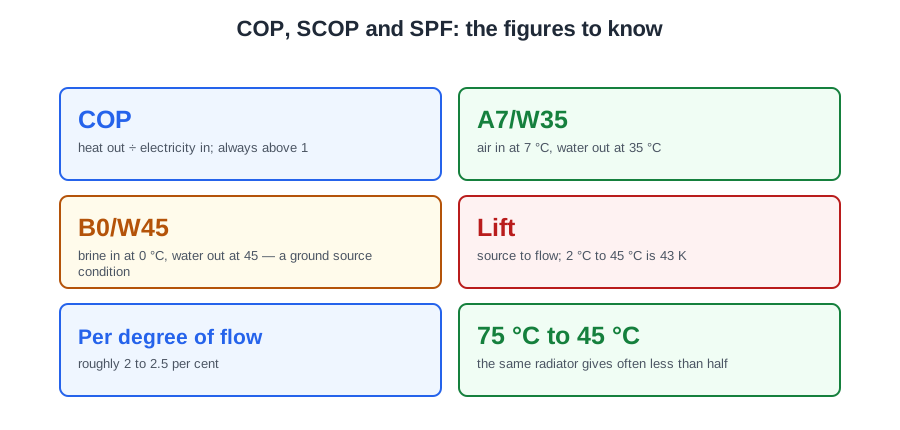
COP = heat output (kW) ÷ electrical power input (kW). A unit delivering 9 kW while drawing 2.5 kW has a COP of 3.6 — 3.6 kW of heat for every 1 kW of electricity it consumes. A working heat pump always returns a COP above 1; if your answer comes out below 1, you have divided the wrong way round.
But the customer asked about winter bills, and the answer is the SCOP, because it is calculated across a whole heating season. A7/W35 is a mild autumn morning, not a British January.
Why it can be "400 per cent efficient"
It can, because a heat pump does not make heat. It moves heat that is already there — in the outside air, in the ground, in a pond — and the electricity only pays for the moving. So the number is not an efficiency in the boiler sense at all: it is a ratio.
| Heat output | Electrical input | COP | What it suggests |
|---|---|---|---|
| 9 kW | 2.5 kW | 3.6 | A sound, ordinary result |
| 11 kW | 3.4 kW | 3.2 | Workable but modest — a fairly wide lift |
A COP without its conditions means nothing. The notation tells you which: A7/W35 means air entering at 7 °C and water leaving at 35 °C; B0/W45 means brine entering at 0 °C and water leaving at 45. The first letter is the source: A is air, B is brine, so B0/W45 is a ground source condition.
Manufacturers naturally publish the flattering condition, which is why two headline COPs are only comparable when the conditions beneath them match.
Lift is what really sets the number
Temperature lift is the difference between the source temperature and the flow temperature the unit delivers. A machine collecting at 2 °C and delivering at 45 has a lift of 43 K. That gap is the work the compressor has to do, and the wider it is, the more electricity is burned for each kilowatt of heat.
Set two identical heat pumps to 35 and 55 °C and the 35 °C system returns the higher COP, because a lower flow temperature narrows the lift. It is not about pump speed, water volume or defrosting.
As a working rule, each 1 °C taken off the flow temperature is worth roughly 2 to 2.5 per cent in efficiency. Twenty degrees is therefore not a detail; it is close to half the running cost.
That rule has a consequence on every conversion from a boiler. A radiator's output depends on the difference between its surface temperature and the room temperature, so drop the flow from 75 to 45 °C and the same radiator emits far less heat — often less than half.
So radiators are oversized on a heat pump conversion to emit the required output at a much lower flow temperature. Nothing to do with water volume, flow rate or a Part L rule on surface area. Underfloor heating, with its very large surface, does the same job by design.
SCOP, SPF and system efficiency
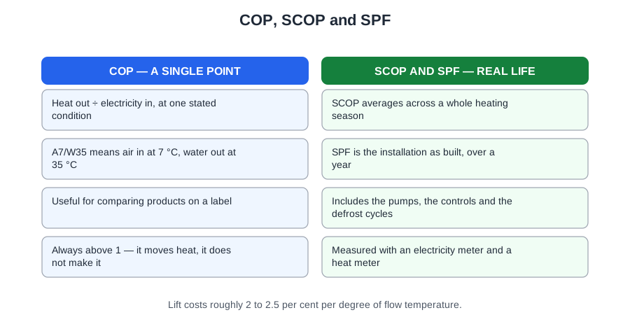
A COP is measured at one fixed set of test conditions. The seasonal coefficient of performance (SCOP) is calculated across a whole defined heating season and a spread of outdoor temperatures. The COP is not wrong; it is a laboratory condition, and quoting it as though it were a year-round result is how complaints begin.
The seasonal performance factor (SPF) goes one step further: the measured seasonal result of the installation as built — the heat it actually delivered over a year against the electricity it actually consumed. It therefore takes in everything a headline COP leaves out: circulating pumps, the brine pump, defrost energy, any immersion heater top-up, distribution losses and standing losses from the store.
SPF is the figure the installer most influences, and that is the point of it. Put two identical heat pumps in two identical houses and one can return a far worse SPF. The most likely explanation is not the refrigerant or the pipe run: it is that one runs at a higher flow temperature with the emitters left unchanged. Same machine, wider lift, worse season.
System efficiency draws the boundary wider still: the heat pump plus its auxiliaries, the distribution, the controls and the storage losses. It explains a fact that surprises people: a good machine badly commissioned, on oversized pipework with a poorly controlled cylinder, can be beaten by a lesser machine installed well.
| Figure | What it measures | Use it for |
|---|---|---|
| COP | The unit at one test condition, e.g. A7/W35 | Comparing machines like for like |
| SCOP | The unit across a whole heating season | Estimating running cost honestly |
| SPF | The installation as built, over a year | Judging the job that was done |
How anybody knows what the SPF actually was
All three figures so far are claims. The SPF is the one that is measured — and it cannot be measured with an electricity meter alone.
The electricity meter records only what the unit consumed; it says nothing whatever about what the unit delivered. Half the sum is missing.
What supplies the other half is a heat meter. It measures the heat given to the system from the flow and return temperatures and the flow rate: the temperature difference tells it how much heat each litre carried, and the flow rate tells it how many litres went past.
The two meters together give the seasonal performance actually achieved — heat out divided by electricity in, over a real year in a real house. That figure does two jobs: it is what an incentive payment is calculated from, and it is what proves the design assumption in service — the one thing that settles an argument about whether a system is underperforming or was simply over-promised.
The ErP energy label supplied with a heat pump exists to let consumers compare the energy efficiency of products consistently, showing an efficiency class alongside figures such as rated output and sound power level. It is not a record of refrigerant charge, not a certificate that the installer belongs to a scheme, and not proof of Building Regulations compliance. A package label can also be produced for the system as installed, reflecting the heat pump together with its controls — a useful reminder that controls are part of the product, not an accessory to it.
🔢 The numbers worth memorising
- COP
- heat out ÷ electricity in; always above 1
- A7/W35
- air in at 7 °C, water out at 35 °C
- B0/W45
- brine in at 0 °C, water out at 45 — a ground source condition
- Lift
- source to flow; 2 °C to 45 °C is 43 K
- Per degree of flow
- roughly 2 to 2.5 per cent
- 75 °C to 45 °C
- the same radiator gives often less than half
- SCOP
- across a whole heating season — the honest running cost figure
- SPF
- the installation as built, over a year, including pumps and defrost
- Measuring an SPF
- an electricity meter and a heat meter
- ErP label
- for comparing products consistently, nothing more
⚠️ Where people go wrong
- Dividing the wrong way round. A COP below 1 is an arithmetic error.
- Quoting a COP without its test condition.
- Comparing two headline COPs taken at different conditions.
- Offering an A7/W35 COP as a winter running cost. That is the SCOP.
- Blaming a poor SPF on the refrigerant when the flow temperature is the cause.
- Judging an installation on the machine alone. System efficiency includes the pumps, controls and store.
- Trying to measure an SPF with an electricity meter. You need a heat meter too.
- Reading the ErP label as evidence of compliance or scheme membership.
- Leaving the radiators unchanged and expecting the data sheet figure.
📝 10-Question Self-Test
Straight from the Level 3 course question bank. Click an option to see whether you got it right — the explanation appears instantly, and there is nothing to submit.
COP = heat output (kW) ÷ electrical energy input (kW), so 9 ÷ 2.5 = 3.6. The unit delivers 3.6 kW of heat for every 1 kW of electricity consumed. A COP will always exceed 1 for a working heat pump — if your answer comes out below 1, you have divided the wrong way round.
COP is a snapshot at stated test conditions — commonly quoted as A7/W35, meaning 7°C air in and 35°C water out. SCOP is calculated across a defined heating season and a spread of outdoor temperatures, so it reflects the reality that an air source unit performs very differently in October and in February. SCOP is therefore the more honest figure for comparing products.
The energy label puts products on a common footing, showing an efficiency class alongside figures such as rated output and sound power level. A package label can also be produced for the system as installed, reflecting the combined effect of the heat pump and its controls rather than the unit alone.
A radiator's output depends on the difference between its surface temperature and room temperature. Drop the flow temperature from 75°C to 45°C and a given radiator emits far less heat — often less than half. Increasing the surface area restores the output at the lower temperature, which is what allows the heat pump to run efficiently.
The loss coefficients set how quickly efficiency falls as the temperature difference widens. Equal optical efficiency means they start level; lower losses mean the curve declines less steeply, so the advantage appears in cold weather and at higher working temperatures — which is exactly the evacuated tube case.
Near the surface the ground follows the air a few weeks behind, so a shallow trench is coldest in the same weeks the building needs most heat. By about 4 m the seasonal swing has gone and the ground holds close to the annual average — around 9°C in northern Scotland to 14°C in southern England at 100 m. The advantage is stability, not extra warmth.
Air-to-air has no wet system and no cylinder, so hot water must come from somewhere else entirely.
On today’s Approved Document L 2021 factors, which come from SAP 10.2, natural gas is 0.210 kg CO2 per kWh and grid-supplied electricity 0.136, so gas is now the higher of the two. It used to be the other way round: the 2006 pair in CIBSE Guide F Table A1.8 was 0.422 for electricity and 0.194 for gas, and the grid has decarbonised since. What this decides is the heat pump question: a heat pump beats a gas boiler on carbon once its seasonal CoP exceeds electricity’s factor divided by the gas one, about 0.65 today against about 2.2 on the 2006 pair. Carry the method rather than the number. Wood pellets are counted at close to zero, not 0.43.
CIBSE gives stagnation, the state where there is continuous high radiation and no heat is being taken off, as over 200 °C for flat plate collectors and 350 °C for evacuated tubes. That is why insulation, seals and jointing are rated against the stagnation temperature rather than the working temperature, and why the fluid has to survive it.
BS 8515 4.1.2.1 states that construction above a certain size based on rainfall for that area provides very limited additional benefit unless stormwater attenuation is intended, and the worked example given with Figure 3 in the simplified approach at 4.1.2.2 shows a four person house needing only about 2.1 m3 in London rather than 3.6 m3 for that reason. Storage is sized at the lesser of 5% of annual yield or 5% of annual demand, about 18 days, not 30, and it is the back-up supply under 3.5 that carries a drought.
Going further: the lessons behind this article
This article is the public answer. Unit 335 of the Level 3 course takes the same ground to the depth the exam and the synoptic assignment ask for, in 2 lessons:
- Coefficient of performance: measuring what a heat pump saves
- SCOP, SPF and system efficiency: the honest figures
- Environmental technology systems: the Unit 335 guide — every article on this unit in one place
- All PlumbMate articles — Level 1, 2 and 3
- The Level 3 course — the whole 8202-35 Diploma